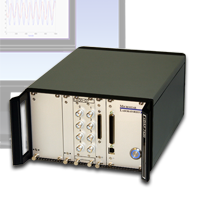
WSM (Wave Synchronization Module)
Wave Synchronization
Related |
|---|
|
The Wave Synchronization Module is available as part of the DAPtools Standard software package for use with Review the manual. |
Sometimes synchronizing measurements simply means keeping things working together. Advanced features such as alignment with a global time standard, accuracy of an atomic clock, or widespread networking are sometimes necessary. But for those other times when a simple stable oscillator is all you really need, that is where the Wave Synchronization Module can help.
You can produce "synchronized" data sets with as little as ±0.00001 radians tracking error relative to the reference waveform signal — that is, synchronization isn't perfect, but almost as good as the reference.
You can maintain alignment despite hazards such as random noise, waveform distortions, frequency drift, or even temporary dropouts in the timing signal.
You can use whatever frequency you happen to have, and it doesn't matter, though you do need to know approximately what that frequency is.
You easily can simplify otherwise difficult measurements, such as Total Harmonic Distortion (THD) or Effective Number of Bits (ENOB), and avoid special custom-designed test equipment.
Sine waves carry rich timing information. Waves change smoothly and predictably, so that every adjustment can reflect the combined influence of hundreds of observations. Furthermore, the abundance of information allows the identification and elimination of offset errors, random noise, and waveform distortions, so that these side-issues do not interfere with stable tracking.
Capturing "timing waveform data" and "measured signal data" side-by-side, a precise mathematical relationship can be constructed on-the-fly. This mathematical association can then be expanded to determine where samples are needed from each measured signal, relative to the timing defined by the reference waveform. With this strategy, you don't need something unusual like a controlled-rate sampling clock and feedback controller to maintain alignment. Once the timing information is known, it doesn't matter whether it resulted from a digital or sine wave timing source, and the TBRESAMP processing command from the Time Base and Time Synchronization Module is used to evaluate signal samples at any rate you want.
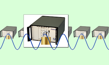
Coarse grained synchronization applications
A 60 Hz timing cycle works well for data collection from sites distributed through a large plant. Values can be reported once per second, 10 times per second, 3 times per second, etc., all of these rates bearing an integer relationship to the 60 cycles per second in the timing waveform, and therefore all easy to coordinate. Very little is critical about this timing, but every station must agree on what constitutes a 60 Hz waveform. If each station tried to generate its own 60 Hz timing signal, variations in frequency or phase from one station to the next would eventually produce inconsistent data.
Perhaps the cheapest and simplest way to share a common 60 Hz timing waveform is to watch a common power system service main. Any devices supplied from the same distribution phase will see the same 60 Hz waveform. This isn't ideal. Power system waveforms can look pretty awful, subjected to phase shifts and distortions due to local loading. However, these things barely matter to the Wave Synchronization Module, and the impacts on timing alignment are a fraction of one power cycle. Rates are locked. No stations can produce too many samples, or too few. With shorter distribution lines, and consistent light loading on those lines, the synchronization is better.
Power harmonics monitoring applications
Power system harmonics due to nonlinear effects of loading can result in stiff service charge penalties, or even dropped service. The first necessary action to control load distortion problems is to observe when the problems occur.
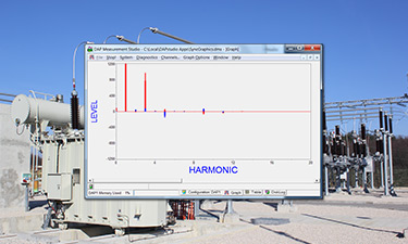
Determining the amount of distortion should be relatively easy using DFT analysis methods — but actually, it isn't so easy. Short term drift in the operating frequency causes the analysis and the actual harmonic frequencies to become misaligned, producing inaccurate results. The following illustration shows a time-plot and a spectrum-plot for frequencies present in a 60 Hz power source voltage waveform, as measured at a wall outlet. The peaks along the spectrum result from harmonic distortions.
Analysis of unaligned data 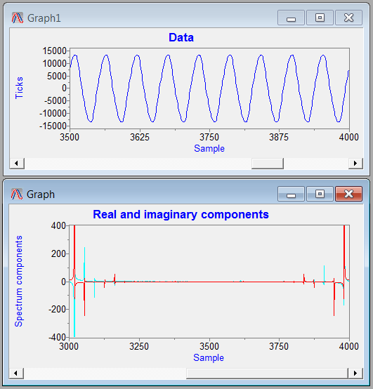
Harmonic distortions have the property that they are spaced exactly at multiples of the fundamental frequency. As you can see in the spectrum plot, however, the curve is "mushy" around each voltage peak. This artificial effect is the result of frequency drift. The problem is that you can't know in advance exactly what frequency to use for the data capture. Schemes such as windowing techniques (see for example standard IEC-1000-3) are often employed, but these remedies are only partially effective, and they introduce their own distortions. Measurement errors in the range of 10 to 20 percent are the norm.
With the Wave Synchronization Module approach, you can use the same waveform data both for the timing wave and for the signal under test. This trick forces the analysis to align to the signal regardless of signal distortion, noise, and continuous frequency drift.
Analysis of aligned data 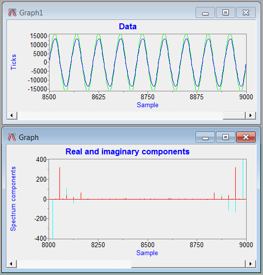
- The number of samples per waveform is maintained almost to perfection, so there is no observable smearing.
- With no smearing hazards, the halfway remedies are unnecessary. Instead of 10% error, you can expect 0.1% error or better.
Total Harmonic Distortion (THD) measurement applications
Distortion effects in a high quality amplifier or converter device are very small. To detect effects so small, it is mandatory to drive that device with a very high quality sine wave, otherwise you could not know whether the apparent distortion was already present before the device under test saw it.
The slightest amount of smearing in the frequency analysis would completely invalidate the results. The usual way to preserve a rigorous alignment between a signal and the sampling is to use specially-designed and expensive equipment that produces both an ultra-pure sine wave and a slaved digital sampler-control clock signal.
Using the Wave Synchronization Module, you still need the precise, clean sine wave oscillator. But oscillator frequency becomes much less critical. Measurements always align precisely, so specialized timing generator equipment is no longer necessary. No windowing or other sorts of fix-ups are necessary.
The following illustration shows the response spectrum measured at a resistor load, driven by a vintage SRS DS360 signal generator. Resistors are supposed to be linear, and the only thing to see in the response spectrum is the original driving frequency.
Undistorted spectrum, linear device 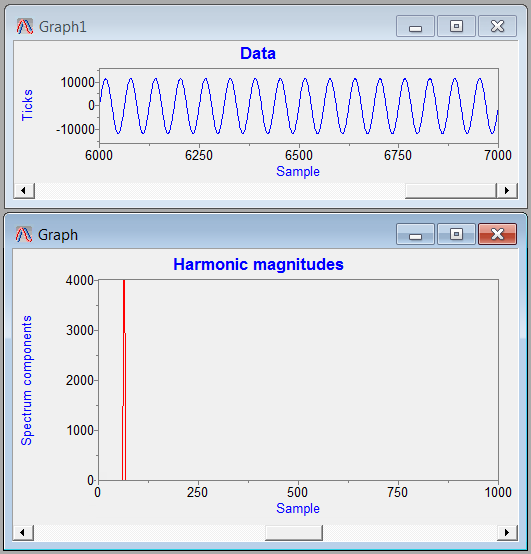
Now a nonlinear element is placed in series with the linear load, deliberately introducing distortions. A distinct harmonic sequence is now visible. We can also see that there are no observable effects on the intermediate frequencies between the harmonics — meaning that smear effects are not present. The test shows actual unbalance and harmonic distortion, not FFT accidents from a poorly designed test.
Spectrum with distortion, nonlinear device 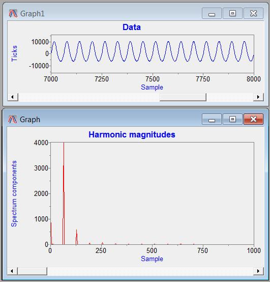
Software configuration example for THD analysis
How hard is it? Basically, you need to add only two additional configuration commands. In addition to that, you can optionally perform the FFT analysis on the xDAP system in real time.
Here is an example showing how the WAVESCAN processing command from the Wave Synchronization Module is configured to perform a THD test. First, the driving signal from the source oscillator is analyzed to extract the timing information.
WAVESCAN( IPipe0, 2.5, 1000.0, pTiming )
- The timing signal raw observations are taken from hardware sample channel 0.
- A 2.5 microsecond per sample interval is chosen, significantly faster than the sample interval to be produced later by resampling.
- The frequency of the driving waveform is 1000 Hz.
- The
pTimingpipe receives the results of the timing analysis.
The timing analysis results are applied to obtain 128000 samples per second from the device response signal, aligned with the excitation signal.
TBRESAMP( IPipe2, 1, pTiming, 7.8125, pResampled )
- The high-rate signal samples come from hardware sampler channel 2.
- There is only one response signal to analyze.
- The
pTimingpipe provides the timing information produced by the WAVESCAN command, as shown previously. - The desired new sampling interval selected is exactly 7.8125 microseconds (128000 samples per second rate) as established by the time base frequency.
- Aligned data samples, ready for analysis, are placed into the
pResampledpipe.
The work of the Wave Synchronization Module is done.
If you wish, the data can then be subjected to an FFT analysis in blocks of 1280 terms. With the sampling rate at 128000 samples per second, and an FFT block size of 1280 samples, frequencies in the resulting FFT will be spaced at exactly 100 Hz per FFT bucket. That means the fundamental frequency of the signal under test, and its harmonics, will be spaced at exact intervals of 10 steps, and the spectrum will cover up to the 60th harmonic. The 1280 samples per block might seem like an unusual size for an FFT, but no problem for the MIXRFFT command, as follows.
MIXRFFT( 1280, FORWARD, RECTANGULAR, pResampled, HALF, POWER, pPowSpect )
- Analyze data in blocks of 1280 points.
FORWARDtransform, from time to frequency spectrumRECTANGULARwindow (no windowing corrections)- Process aligned data from the
pResampledstream. - Since the spectrum of a real-valued stream is redundant, post-process raw power spectrum to produce a HALF-size output block.
- Post-processing results are the values of POWER density at each frequency.
- Spectrum terms are delivered through the
pPowSpectdata pipe.
Even better results can be obtained by averaging a number of spectrum blocks together, to reduce random effects.
Technical performance
| preserved flat band width | 40% of Nyquist frequency at original hardware sample rate |
| preserved band flatness | ±0.00025 dB (equivalent to ± 1 LSB) |
| typical phase alignment | better than 0.00001 radians short term |
| long-term frequency error | 0.0 |
| reference frequency range | 1.0 to 1000.0 cycles per second |
More information is available in the Wave Synchronization Module: Command reference and application guide.
The Wave Synchronization Module is distributed as part of the DAPtools Standard software.