Configurable Chirp Generation for Sonar Surveys

Introduction

A typical marine bottom survey in deep water might study sediment accumulations to a depth of 30 meters or so. A "fish" device is trawled below a ship, sending out sonar pulses. These are not simple pulses, rather, they are complex pulses with waveforms having controlled spectral content, and with a well-selected pulse shape. The pulses will echo back from discontinuities between material layers where density changes. By analyzing the distortion and time delay of the return echoes, the properties and dimensions of the layers can be mapped.

The shapes and frequency content of the pulses matter. Depending on the study, the signals might be configured differently for best resolution, best directionality, best penetration depth, etc. While DAP boards and the DAPL systems are not complete sonar measurement system solutions, they offer hardware and software features useful for signal shaping, signal generation, and data capture for these systems.

Pulse Shapes and Swept Waves

Frequencies propagate differently in different materials. The energy of some frequencies is absorbed faster by certain materials, yielding less return information. Some frequencies result in less echo distortion and better correlations in the analytical results. For these reasons and others, it is desirable for survey signals to cover a band of frequencies. Information you can't get at one frequency might be readily available at another.

A swept wave or chirp signal has a time-varying frequency, and provides the right kind of spectral coverage. Piezoelectric transducers for survey applications can typically cover a frequency band of about 1000 to 15000 Hz [1]. The following illustrates a single chirp sweep.

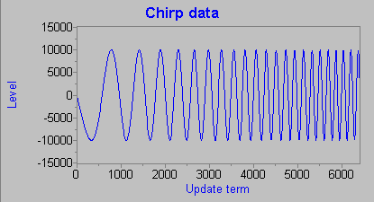
Chirping has some big advantages over continuous signals. If you have the same frequencies transmitting all of the time, one waveform will look like another. You have lots of information for identifying frequency content, but you can't isolate time events producing that frequency content. If you reduce the chirps to short time intervals, you improve the time resolution dramatically, though it is harder to distinguish the frequency content in the return signals.

The abrupt edges of the squared pulse in the previous illustration has some negative side effects. In the echo results, you can't tell which effects come from the signal and which come from the artificial edge discontinuity. This is basically the same problem as frequency anomalies from chopping a signal block into pieces for performing an ordinary FFT analysis — are the observed effects actually due to the signal, or due to chopping it? To avoid these unresolvable problems, windowing techniques used for FFT analysis are helpful.

In sonar applications, the Blackman-Harris window [2] is the conventional choice. After applying it to shape the chirp pulses, the chirp shape will look like the following.

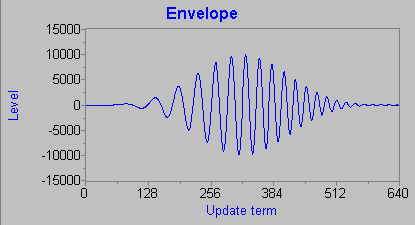
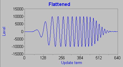
While the Blackman-Harris window has good properties for low distortion and good sideband rejection, you can see that it severely attenuates more than half of the tone burst. It also has poor properties for local discrimination. You can partially compensate for range loss by extending the frequency range at each end. Experiments have demonstrated that some flattened alternative pulse shapes [3] provide better resolution with an acceptable penalty in sidebands and noise. These pulses have smoothed transition edges but flat central regions.

Generalizing the Chirp Window Properties

The flat-topped "sine squared transition" shapes and the Blackman-Harris window shapes can be generalized into one envelope family by introducing two shaping parameters:

1. The plateau width. The flat-topped pulses can be considered a three-part composite shaped, with an up-transition zone, uniform flat zone, and symmetrical down-transition zone. The plateau width parameter determines the width of the flat region. The shaping of transitions can be produced in two ways (that are in general not equivalent).
   • Convolve a wide rectangular window with a narrow shaping window.
   • Split a narrow window shape into two parts, assigning the left half to shape the rising transition, and the right half to shape the falling transition.
   The second scheme was implemented, but changing to the other would not be difficult.
2. The transition shape. The "sine squared" transition shape used in the field studies can be produced by choosing the narrow window to be a von Hann window. Generalizing the window would allow for adjustable shaping of the transitions.

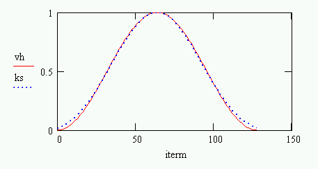
A cosine series representation of window shapes is feasible, but dealing with the multiple configurable parameters is inconvenient. We can observe that a Kaiser window is a continuously adjustable window family that can provide high quality windows based on a single shaping parameter. For example, the following plot shows the Kaiser window with parameter 3.85 superimposed on the conventional Blackman-Harris window. It is hard to believe that they are not generated by the same formula.

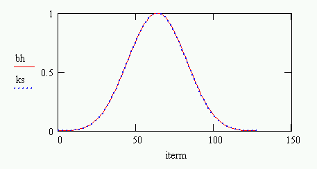
The Kaiser window does not produce the same degree of matching to the von Hann "sine squared" shape. The Kaiser window with parameter 1.86 seems to match well in the central interval where magnitudes are larger, but not so well at the tails. This makes the window shape somewhat like an intermediate between the von Hann and the Hamming windows, which is not necessarily a bad idea.

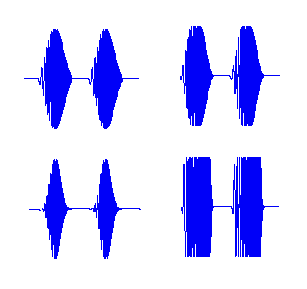
The Kaiser window and plateau width parameters can be adjusted to produce a variety of chirp envelope shapes.

Generating Sonar Pulses with DAPL Processing

The real-time signal processing for the sonar system can be broken into five sub-problems, and the DAP can help with at least four of them.

1. Configure and establish the frequency sweep for the chirps.
2. Generate and apply envelope shaping to modulate and isolate chirps.
3. Issue the drive signals for transmitting the chirps.
4. Monitor the echo responses.
5. Perform post-processing and display of captured data.

The details will be different for each application, of course, which is fine, because the DAPL system is completely configurable.

Generating the swept frequency waveform

The CHIRP command produces frequency sweeps at a uniform amplitude. It runs as embedded processing on the Data Acquisition Processor board. It allows you to specify the low and high frequency range limits for the sweep, the sweep function shape (the usual choice is a linear sweep), and the length of the sweep. The length and frequencies are expressed as numbers of samples, so specify them based on the selected sampling rate.

Let us suppose that the lower range of the sweep is 1.25 kHz and the upper range of the sweep is 12.5 kHz. We don't want to worry about strange sample-and-hold artifacts in our drive signals, so we will drive at a high oversampled rate of 200 kHz. That allows 16 samples per waveform at the highest frequency, 160 samples per waveform at the lowest. This should give accurate transducer tracking through the entire range.

One more decision: How long is the chirp pulse? We probably don't want to be transmitting at the time that the return echo comes back. Let's suppose that we select a chirp duration of 32 milliseconds, making this less than a two-way return delay of 40 milliseconds. The 32 millisecond chirp corresponds to a group of 6400 samples at a rate of 200000 updates per second.

The CHIRP processing command to generate a linear, low-to-high frequency sweep would be configured in the following manner.

   CONSTANT  AMPLITUDE LONG = 32700

   PDEFINE  GENERATOR
     CHIRP("linear", "unidir", AMPLITUDE, \
        6400, 160, 16, 0.0, PCHIRP)
     ...
   END

At runtime, the CHIRP task generates a stream of repeated chirp cycles and places them into the PCHIRP pipe.

Shaping the chirped pulses

The DAPL system does not provide processing commands for specialized functions such as sonar envelope shaping, but that is not a problem. The DAPL system is designed to be extended, using the Developer's Toolkit for DAPL. We have done this to build the ENVELOPE command.

Besides taking the stream of chirps from the CHIRP command and applying a modulating envelope, the ENVELOPE command can also inject any desired quiet time between pulses, making the operating cycle length adjustable independent of the chirp length. The total operating cycle must allow enough time for the two-way transit, also allowing for delayed responses from deeper features.

For example, to generate a 32-millisecond burst at 200 thousand sample per second update rates, that is 6400 samples. If there is a 40 millisecond two-way transit time plus a 50 millisecond interval for observing return echoes, that is 18000 output updates in the complete cycle. A configuration using a Kaiser window shaping parameter of 3.85 and a 50% plateau width would use the following configuration.

  PDEFINE  GENERATOR
    ...
    ENVELOPE(PCHIRP, 6400, 18000, 3.85, 0.5, PBURSTS)
    ...
  END

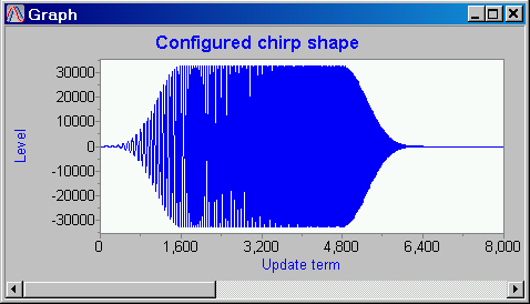
The Graph window in the DAPstudio application can be used to observe this wave shape.

Driving the pulsed waveforms

The chirps and quiet times form a repeating cycle. These values can be pre-computed, placed into a buffer, and issued under control of a crystal oscillator for precise update timing. The desired 200000 updates per second is configured by setting the clocked update interval to 5 microseconds. The digital to analog converters drive the transducer to produce the desired signal under hardware control.

This is an easy configuration for a Data Acquisition Processor. The output configuration will look something like the following:

  ODEFINE   TRANSMIT  1
    SET OP0  A0
    TIME     5
  END

To send the data [4], just copy it to the output channel pipe from the processing section.

  PDEFINE  GENERATOR
    ...
    ...
    COPY(PBURSTS,OP0)
  END

Monitoring the echo responses

The returned chirp echoes are sensed and recorded. There are various clever things that can be done with input sampling, but assume here that everything is sensed and recorded as one stream. Output chirps will have a lot of signal energy and will overdrive the input amplifiers, so measurements will not be meaningful while bursts are transmitting. But burst times are clearly identifiable in the data sequence, which is helpful for validating the input timing and output timing. The input sampling and the output updating use the same time base[5], so input samples and output samples relate one-for-one.

    IDEFINE  LISTEN
      CHANNELS  1
      SET  IP0  S0   10
      TIME      5.0
    END

Code Availability

A downloadable binary code module is available upon request. This module contains both the CHIRP and the ENVELOPE commands. Full details about using the commands is provided with the module. Loading the module makes the two processing commands available to define embedded processing tasks, as illustrated by the examples.

Is That All?

No, that's just the beginning. With the Data Acquisition Processor spooling pre-computed data to output and capturing response data at a mere 200000 samples per second, that means it is only operating at 25% of capacity [6]. Data Acquisition Processors can crunch through FFT transforms while running at 100% capacity. Since sonar detection can involve some tricky digital filtering, correlation, or wavelet analysis, this means that you have a computing resource that you can use to advantage for some of the computing that must be done in real time.

Conclusions

Data Acquisition Processors, the DAPL system, and the Channel Architecture provide integrated resources that make some aspects of sonar survey applications surprisingly easy to implement. The DAP operates on the bus of the host processor, so it is easily integrated into an advanced processing system. It provides all of the signal generation, data capture, and logging facilities. The details of real-time signal generation and capture are covered, so your application software operates at a higher level and does not have to deal with them.

We have shown how to generate chirp signals with configurable sweeps and configurable windowing shapes. If it turns out that the advanced technique of today is obsolete tomorrow, that is not a problem. The DAPL system is meant to be extended, and the modular extensions can be independently modified. You won't need to rebuild your entire software system, or replace all of your hardware components to implement new methods.

Footnotes and References

1. For example the Neptune T135 wide band sonar transducer. [Return to the text.]
2. The 4-term Blackman-Harris window gives excellent sideband suppression. For t in the interval 0 to 2 pi, the window formula is:

    0.35875 - 0.48829 cos(t) + 0.14128 cos(2t) - 0.01168 cos(3t) 

   This window was recommended in the study "Spatial and Temporal Pulse Design Considerations for a Marine Sediment Classification Sonar," S. G. Shock, L. R. LeBlanc, and S. Panda, IEEE Journal of Oceanic Engineering, v 19 n 3 (1994): pp 406-415. [Return to the text.]
3. "Chirp sub-bottom profiler source signature design and field testing," Martin Gutowski, Jon Bull, Tim Henstock, Justin Dix, Peter Hogarth, Tim Leighton, Paul White, Marine Geophysical Researches, v 23 (Kluwer Academic 2002): pp 481-492. They tested various combinations of sweep functions and envelope shapes for mapping features along a well-studied seismic line. [Return to the text.]
4. Advanced applications can bypass the COPY task and stream data to the output updating directly from the ENVELOPE command. [Return to the text.]
5. We have glossed over a few details about timing here. You can use some special hardware configurations to more precisely align the input and output sampling events. Once established, the time relationship between channels remains the same, all the time, every time. It's okay, call us and we'll help you get this set up. [Return to the text.]
6. Advanced users will use the CYCLE command to regenerate the output sequences, effectively releasing most of the 25% of processor capacity back to the DAPL system for other processing. [Return to the text.]

Return to the DSP page.

© 1994-2024, Microstar Laboratories, Inc. All Rights Reserved.
webmaster@mstarlabs.com 888-678-2752 (US/Canada) or +1-425-453-2345