Online Self-Tuning PI Controller

Introduction

(View more Control information or download preliminary software modules.)

This note describes an experimental PI controller augmented with automatic self-test and self-tuning features. While not a fully commercial implementation, this controller has some interesting features that might make it useful in its present form. This might be considered an advanced topic but don't worry, you don't need the mathematical details to use it.

With a PID controller, or particularly with a PI controller, there aren't many gain terms to adjust — how hard can it be? Plenty hard, as it turns out. Controller gains always appear in combination with unknown plant parameters, so the closed loop performance defies conventional mathematical analysis. Usually, the reason for PID control is that you really don't have a system model, nor the time to derive one. Maybe all you have is a general level of confidence that PID "should be good enough for this kind of system." How do you put that into an equation to predict good controller gains?

Lacking an accurate model, lacking even an approximate model, you might try to "get by" using historical loop tuning rules. That's fine, but the apparent simplicity hides some serious disadvantages. You are required to take the system offline for some tricky frequency response tests that relate only indirectly to the objectives you are trying to achieve. To tune the control loop after it goes online, you must either resort to "trial and error" or repeat the offline measurement process.[1]

Rather than trying to specify system behaviors in terms of various analytical artifacts such as critical frequencies and phase margins, you might decide to concentrate on results. This approach leads to a performance measure function, but what is the relationship between the performance measure and the adjustable gains? In a way, this is the same problem, but pushed to a different place and still difficult.

The Iterative Feedback Technique [2] offers a new approach for adjusting the gain parameters for low order linear controllers such as PID. Rather than trying to estimate unknown plant parameters, it circumvents the problems in three ways.

The terms in which interacting control and plant parameters appear together become measurement terms, substituting observations for theoretical analysis.
Special input sequences are constructed as test signals, based on previous measurements, to remove dependence on unknown parameters.
The method does not determine specific gains to apply, but it does produce incremental adjustments to improve the existing gains.

Self-tuning PI controller

This note describes a variation of the Iterative Feedback technique, reduced for the special case of a PI controller regulating a fixed level, but extended for online operation.

The dilemma of online tuning is that you don't want to disturb the system too much because that interferes with production. On the other hand, if nothing changes, tuning is impossible because you can't observe the dynamic loop response.

The original Iterative Feedback method requires large disturbances inconsistent with online operation. The modified controller uses a superimposition principle, with small injected test signals that ride on top of a fixed setpoint level signal. In fact, any setpoint adjustment will abort tuning activity, so you cannot use this method while continuously tracking a changing setpoint level.

The modified controller operates on an adjustable cycle. Each tuning test cycle is followed by a period of undisturbed operation using the adjusted controller gains.

A demonstration

Before getting into the technical details, here is a quick demonstration of what it can do.

The self-tuning process was incorporated into the PIDZ command [3] to make a self-tuning variant, PIZST. The derivative gain term is not tuned but neither is it disabled. It remains at its initial setting, as if the derivative feedback path was part of the controlled plant. You can obtain classic PI control by setting the derivative gain term to zero.

The red trace in Figure 1 below shows the response of a plant to a step disturbance using the initial gains, before automatic tuning. The plant has a dominant and secondary lag plus pure time delay response (but of course the controller does not know anything about this). You can observe that the magnitude of the test disturbance is about 200 converter counts, which is less than 1% of the full scale level of about 32000 counts. You can also observe that the response is sluggish, taking about 40 controller updates to settle.

Figure 1 - Before Tuning
step response with initial gains

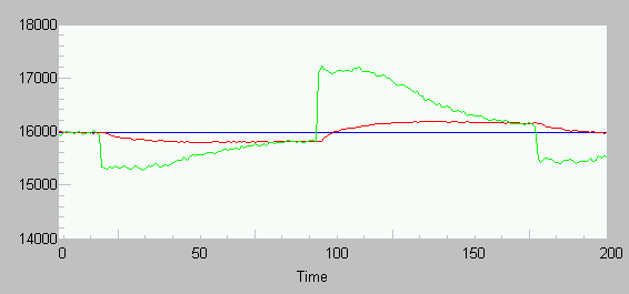
KGAIN  = 4.000
TI     = 0.350
TD     = 0.00001
ZGAIN  = 0.800
TSAMP  = 0.05

Figure 2 shows the same simulated system, after 250 incremental gain adjustments. The response now settles in roughly 15 controller updates. The PI controller has "tuned itself."

Figure 2 - After Self-Tuning
step response with initial gains

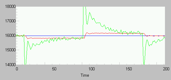
KGAIN  = 10.2224
TI     = 0.2620
TD     = 0.00001
ZGAIN  = 0.9973
TSAMP  = 0.05

Notations and equations

We need a reference model to describe the control loop action, even if we don't know all of the model parameters.

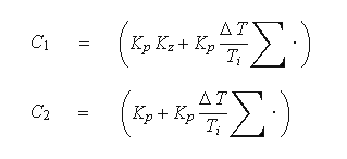
The controller action is organized into two control paths, C1 describing the gains applied to the command input signal, and C2 describing the gains applied to the feedback signal. Controller gains are adjusted but always known precisely. The combined effect of these two "filters" equals PID control. The plant model P is unknown and includes any derivative feedback effects if present.

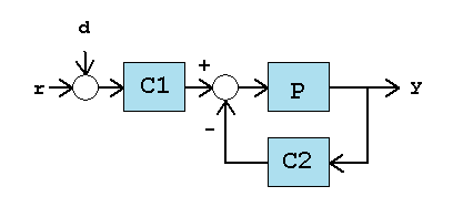
The transfer response to the command signal r and to the disturbance d is described by the following familiar command-to-output transfer function T.

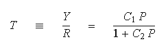
It is presumed that the plant is approximately linear, and there exists a constant level on the command input that will sustain a desired output level, so that a stable PI control loop will eventually settle to hold the command level r on the plant output. We make use of this fact for the superimposition principle.

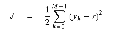
Performance measure

The Iterative Feedback approach uses a performance measure for describing a "good" PID loop tuning. We use an average of the command tracking error squared, for a performance evaluation with minimal complexity. The tunings tend to cancel disturbances efficiently, but at the expense of some overshoot.

Performance measure gradient

A controller based on the PIDZ command [3] has four adjustable parameters: loop gain, command path gain, integral gain, and derivative gain. The derivative gain term is ignored by the tuning process.

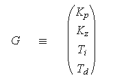
The gradient of the performance measure describes how much performance changes in response to an incremental change in the gain parameters. Because the derivative gain is not adjusted, its sensitivity term is fixed at zero.

Observing that changes in the plant output level appear directly as changes in the tracking error, we can differentiate the performance measure with respect to parameters to obtain the following gradient expression.

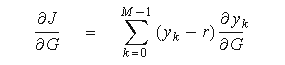
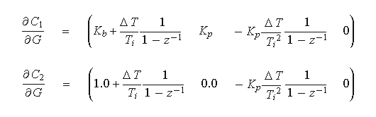
To obtain the first term, we can run an injection experiment, injecting disturbance sequence d_k and observe the tracking error y_k-r that results. For the second term, the general derivative expressions [2] reduce to the following for the case of a PI controller.

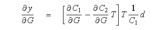
Some observations about this expression:

The 1/C1 filter is the inverse of the PID gains on the input path. We can derive this discrete filter by inverting the equation of the discrete PI controller, producing a simple digital filter in the form
```
      y₀ =  y_-1 K1 + (x₀-x_-1) K2
  
```
where K1 and K2 are directly determined from the current controller gains.
The last term of the gradient expression is the 1/C1 filter applied to the predetermined input disturbance. Knowing the PID gain settings, we can analytically pre-compute this sequence.
The T notation is the transfer function of the closed loop system. We do not know what this is because the plant P is unknown. But we can observe the response of the closed loop to a known injected disturbance 1/C1 d to observe response T 1/C1 d in combination.
The expression in square brackets contains an additional transfer function term T. This presents the same kind of dilemma again. We don't know what T is, but we can observe its response to the disturbance T 1/C1 d we observed in the previous experiment. This process of taking the output of the previous experiment and feeding it back into the input as a new test signal motivates the name Iterative Feedback.
The gradient expression then consists of a combination of the known sensitivity vector terms with the observations from the direct injection experiment and the iterated injection experiment.

Limitations of gradient tuning

Initial gains must be specified. It is usually easy to guess safe and stable gains. For the systems where this command might be used, selecting gains that are a little low is sufficient to ensure stable operation.

The gradient expression produces a direction, not a magnitude. To determine how much to change the gains in the direction indicated by the gradient, an appropriate (but somewhat ad-hoc) "learning rate" factor is applied.

Gradient methods have a well-deserved reputation for starting slow and getting slower. Near an optimum, the adjustments approach zero. As a partial compensation for this inherent slowness, the PIZST command uses a variable step method in an attempt to accelerate convergence.

Disturbances can occur during tuning or during normal operation. If disturbances occur, they will influence the tuning results short term, and gain values will "wander" in the neighborhood of the optimum settings. For normal systems, small gain variations have no significant impact on loop stability.

Configuring a self-tuning loop

The self-tuning PID processing can be configured by substituting the PIZST command for the PIDZ command[3].

  CONSTANT   DISTSCALE    FLOAT = 0.005
  CONSTANT   ADJSTEP      FLOAT = 0.00025
  CONSTANT   UNDISTURBED  WORD  = 4000

  PIZST( PSET, PIDIN, \
         KGAIN, TI, TD, BGAIN, TSAMP, \
         PIDOUT, LOWLIM, HIGHLIM, \
         DISTSCALE, ADJSTEP, UNDISTURBED )

The gain parameters are the same as in the original PIDZ command, except they specify initial gain values only.

The three new PIZST parameters are:

the magnitude of the injection signal, as a fraction of full output range
(Careful, this is not the same as a fraction of the operating level.) A value of 0.005 to 0.02 is typical, depending on how much disturbance your process can stand.
a "learning factor" for converting the gradient into gain adjustments
It is typically around 0.0001 for a disturbance level of 0.01. You will have to experiment to find a level that produces reasonable, slow but steady improvement. If you decrease the injection signal, you might need to increase the learning factor to preserve the learning rate.
the number of samples of "normal undisturbed operation" between tuning experiments

Conclusions

The PIZST command should be considered a work in progress, not a finished product. Even so, it might be useful in its current form. If you would like to try it on your DAPL system, you can download a copy. It is most likely to be successful with process regulation applications (pressure, temperature, flow rate, etc.) which have lowpass frequency characteristics with lagging phase shift.

There are helpful or mandatory ways this processing might be extended — let us know what you think.

Learning and scaling factors should be easier to use.
Extend the analysis to tune the derivative term as well.
Modify the performance measure to reduce transient overshoot.
Near optimum, the disadvantages of the test disturbances outweigh any possible benefits from further performance gain. Reduce tuning activity until a need for it is apparent.
Provide supervisory control. Allow tuning to be enabled or latched. Allow manual overrides of gain settings.
Provide observability. Make it easy to obtain test results on demand. Make it easy to observe the current gain settings.

While there are plenty of technical questions related to what should go into the package, making the package is not a problem. The channel architecture of Data Acquisition Processor systems provides all the basic features: fast, accurate signal conversion, configurable data processing, task independence, and CPU power for reliable real-time response.

Self-tuning controls are not the perfect solution for every application, but they might be near-perfect for some. If you can trust a controller to maintain itself near optimal performance, that means productivity gains plus reduced maintenance effort. It would be great if you could trust it to work perfectly all the time, every time. As a practical matter, however, it needs to prove itself with each application. If it does work well, that means one less controller needing constant attention, leaving time for working on the more difficult problems.

Footnotes and References:

The article A Self-Testing PID Loop on this site describes a command that helps to automate the measurements, but it won't make the results any better.

"Iterative Feedback Tuning: Theory and Applications" in IEEE Control Systems, August 1998, pp. 26-41.

PIDZ - A PID Controller With Zero-Shaping on this site. The supplemental "Z" gain term provides some additional control of transient overshoot in response to setpoint command changes.

Return to the Control page.